Solving ODE/PDE with Neural Networks

Differential equations and neural networks are naturally bonded. The best paper “Neural Ordinary Differential Equations” in NeurIPS 2018 caused a lot of attentions by utilizing ODE mechanisms when updating layer weights. On the other direction, there are also many research using neural network approaches to help investigate differential equations such as “Deep learning for universal linear embeddings of nonlinear dynamics”, “DGM: A deep learning algorithm for solving partial differential equations” or “Solving Irregular and Data-enriched Differential Equations using Deep Neural Networks”. In this post, I will make two toy examples to show the very the basic idea of using deep learning method for solving differential equations.

The basic idea

To put it in a simple and rough way, differential equations are equations like $L u = 0$ subject to boundary/initial conditions $ f(u; p) = 0$ on some domain $\Omega$. $L$ is certain differential operator (maybe with respect to time or spacial coordinates) such as $\partial t + \Delta$. Our goal is find a ``nice” function $u$ well defined on $\Omega$ that satisfies these equations at the same time. This task is NOT easy, work/research that has been continuing for centuries to develop mature theotical and numerical methods to study the behavior of these equations as well as their possible solutions. If your major is with STEM discipline, you certainly can not escape from this topic in your course work.

Long words short, the neural network can come into play in this yard is because of at least two reasons.

• One is the fact that universal approximation theorem states that “simple neural networks can represent a wide variety of interesting functions when given appropriate parameters”.
• The second reason is that modern computation framework such as Tensorflow or PyTorch allows the user to get the numerical differentials of given variables quite easily once the computatio graph is correctly built.

For example, if $y = 2x^2$, with some easy calculus knowledge you know $\frac{dy}{dx} = 4x$. You will then know every exact value of this derivative when the actual value of $x$ is given, e.g. $\frac{dy}{dx}|_{x=1} = 4$. The number 4 is essentially what you can get from these computation frameworks if you query the first order derivative of $y$ w.r.t $x$ and feed the value 1 to variable $x$. Now with useful tools as these, the solution of differential equations can also be addressed as an optimization problem: the network $\phi$ should learn parameters $p$ so that the object function $||L \phi(p)|| + ||f(\phi; p)||$ is minimized. $||\cdot||$ is some norm or metric used to measure the error. Some commonly used ones are mean sqaured error (MSE) or mean absolute error (MAE). One could also use a weighed sum to balance the equation loss $||L \phi(p)||$ and the boundary condition loss $ ||f(\phi; p)||$.

Now Let’s play some toy examples.

1d example

$\frac{dx}{dt} = -x$ and $x(0) = 1$

First, we need to think about what data to feed into the neural network. It is easy in this example, we can just feed grid points or randomly selected points (x, t): (1, 0), (1, 0.2), (1, 0.4), (1, 0.6), … Second, we should consider what needs to be done to enforce the initial/boundary conditions. There are at least two ways:

• Feed points at the boundary consistently to the network during training. This method is simple, but the points needed grows exponentially with the growth of dimension and the training may not be stable if these points are not properly selected.
• Construct a solution template so that initial/boundary conditions are automatically satified. This method requires some human genius. In this toy example, the template is easy, one can set the form of solution: $x = x_0 + t\phi$. In this case, only the equation loss will remain in the object function for optimization.

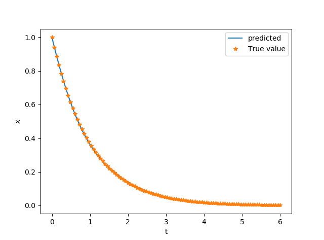
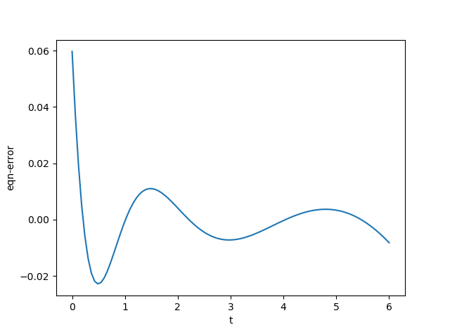
Once the network is built (here a simple MLP with only one hidden layer is used for $\phi$) and training data obtained, we can train it to see how it performs. In this toy example, the training should be done with <1s on your laptop. The flowing picutures show the prediction from the network (left) and the error term of equation, i.e. the value of $\frac{dx}{dt} + x$. Not too bad, and you can certainly improve it yourself. The code for it can be found here.

2d example

Now let’s work on the Laplace equation

$\Delta u = 0, u = u(x, y)$

with boundary conditions

$u(1,y) = u(0, y) = u(x, 0) =0$ and $u(x,1) = \sin (\pi x)$

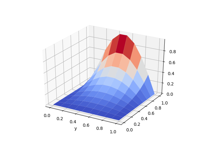
on unit square $[0, 1] \times [0, 1]$. The solution template here will be a little more complicated as

$u = y\sin(\pi x) + x(x-1)y(y-1)\phi$.

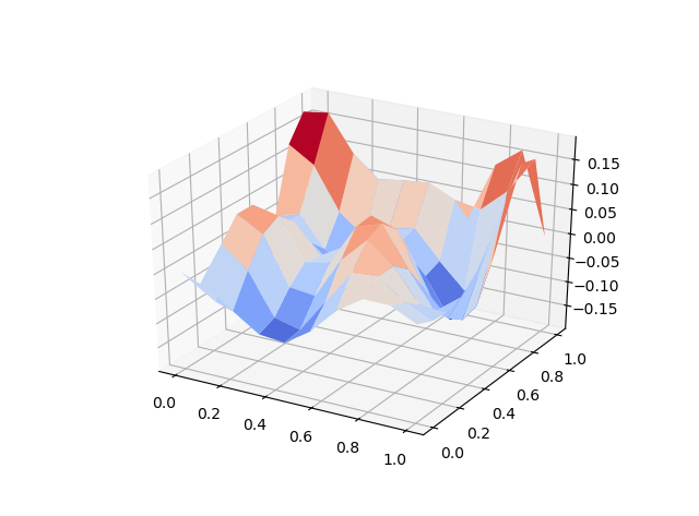
Again, you can use grid points or randomly selected points (x, y) in the unit square as training data. The training time may be a little longer depending on your training data size. The following example only uses about 100 grid points, 2000 epochs and the training completed within seconds. (check here for the code). Predicted solution is shown on the left, the equation loss is plotted on the right. The performance can be improved with more training data or deeper network.